Interpretation of Lidar Output

In this section, we begin to tackle the interpretation of Lidar imagery by inspection (finally!). In fact, there is an incredible amount of information you can gather from the Lidar output without further use of computers or algorithms. This can be accomplished by training yourself to recognize features that can be explained by basic knowledge of the atmosphere.

To quickly reach a certain topic, click on one of the 8 sections listed under the "Interpretation of Lidar" navigation menu on the right.

General Concepts

In the simplest of ways, how do we “read” lidar imagery? It is important to note that lidars are in-situ field instruments, and that they do not capture the evolution of one particular feature over a certain distance. That is to say, they provide a Eulerian frame of reference for output. What we see on the output can be thought of as a sequence of “snapshots” or “slices” of the atmosphere, stitched together to make a complete photo of what occurred over one particular point on the ground throughout the course of a day.

To begin, let’s look at a randomly selected day from the CORALNet-UBC catalogue of lidar imagery at 1064 nm, as shown below:

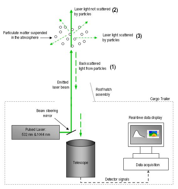
First, note the axes and colour scale that are used. On the horizontal x-axis is the time of day (shown here in local time, PDT), and on the y-axis is the altitude up to 15 km above ground level. To the right you will find a colour bar denoting the amount of backscatter ratio (or for simplicity, “backscattering”). Note that this is a logarithmic scale, where low values (cool colours) denote low backscattering ratio, and high values (white/warm colours) denote high backscattering ratio.

Backscattering ratio is defined as the backscattering by particle vs. total scattering, or as the scattering of light back towards the emission source (the lidar) vs. the scattering of light in another direction. Recall that these processes were depicted and described in the schematic drawing of the lidar setup.

Think back to the Lidar Basics section when we stated (generally speaking) “the more aerosols, the more backscattering”. Knowing this, you can probably make a good guess of what is being capture in the figure above! There are 4 particular “features” of interest (denoted by letters):

1. From approximately 00:00 to 15:00, at ~6 km above ground, there is maximum backscattering. Of course, this is a cloud deck passing over the station! Mid- to lower- level clouds usually correspond to areas of maximum backscattering (white), logically, since clouds are composed of countless water droplets (aerosols). The altitude at which the high backscattering is recorded can give you an idea of what category of cloud is present.
2. Contrastingly, from 15:00 onwards, there is low backscattering (black-blue tones), which indicates a clear atmosphere above ~1.5 km.
3. Taking the entire lower portion of the output below ~1.5 km as the featured “C”, you can also see that there are intermediate to high values of backscattering from ground level to ~1.5 km throughout the entire day. The higher values around ground level can be attributed to (presumptively) anthropogenic aerosols created over the course of a day or advected into the area. These intermediate to high backscattering values at ground level are observed as haze.
4. From approximately 11:15 – 11:30, there is a black area extending the entire depth of the atmosphere. Be cautious, this is not to be confused with feature B! In fact, the lidar has shut off at this point in time, for either maintenance, or due to the passage of objects overhead. (Note: We know that this is not due to rainfall by looking at the ancillary data from the lidar’s meteorological tower).

Next, to piece together the picture a little better, imagine that you are standing on the “ground” at 0 km of the output and “looking up” into the atmosphere at a particular point in time. What features will you see? Let’s take two examples from the same image above :

1. At 06:00, we know that feature A is located directly above the station (aloft). There is also feature C at ground level. Thus we can expect overcast skies, with haze at ground level.
2. At 18:00, feature B is located aloft, while there is still high backscattering at ground level (C). Thus we can expect clear skies with haze at ground level.

It is easy to check if our assumptions are indeed correct. Accessing photos taken at ground level (e.g. from KatKam) corresponding to the times of interest confirm our interpretation, as illustrated below:

KatKam images for (i) 06:00 partially overcast skies and (ii) 18:00 clear skies, July 20th, 2010. Note the haze in each, as the background landscape is obscured.

Cloud-base Height

An important result follows from the example discussed above. Note that feature A can be roughly interpreted as “a thick cloud cover”. But what about the atmosphere above it – can we deduce the distribution of aerosols there?

Notice that from ~ 06:00 – 13:30, there is a large black region above A. Again, this is not to be confused with clear skies (B) or lidar shut off (D). In fact, the black region here means that the lidar signal was sufficiently attenuated.

With thick cloud cover, nearly 100% (white) of the original lidar pulse is backscattered, since there are “a lot” of aerosols (and, also due in part to the spherical nature of the cloud droplets, discussed below). Thus, nearly none of the signal is able to pass directly through the cloud cover to potentially backscatter from other aerosols or cloud layers aloft.

Because of this, the cloud-base height is the most reliable information derived from ground-based Lidars – the lidar signal is usually attenuated before the cloud-top is reached. From the raw lidar output, automated algorithms are often applied to detect cloud-base height and vertical cloud distribution or various cloud layers or regions of clear atmosphere in between, where possible.

Furthermore, any backscattering measurements through the depth of the atmosphere can be severely impeded by fog. Since fog is “cloud at ground level”, a maximum backscattering can be observed in the lower portion of the atmosphere. On the 532 nm channel there are “no measurements” (black), and on the 1064 nm channel, the backscattering during periods of fog often appear as maximum backscattering “noise”. Again, this is not to be confused with lidar malfunctioning and/or shut off. We can verify this by looking at ancillary data provided by the lidar’s meteorological tower. An example of a fog event and its confirmation is provided below.

A fog event as captured by the CORALNet-UBC lidar station. The 532 nm channel (upper left) shows mainly "blank/black" output, whereas the 1064 nm channel shows "noise" of maximum backscattering. Though the black portions of the 532 nm may lead us to assume that it is raining, and the 1064 nm may lead us to assume that there is a lidar malfunction, neither is correct! If we look at the ancillary data from the lidar's meteorological tower, the relative humidity is close to 100% (center left, blue line) and there is no precipitation (center right, rain rate = 0, or "Raining = No"). Thus what we are capturing is indeed fog! This is illustrated in the KatKam photo of the same day at (e.g.) 15:00.

Boundary Layer Structures

Not only can lidar help identify features of the Planetary Boundary Layer (PBL), but these features will also influence the dispersion of aerosols and air quality. Courses in meteorology often examine the classic schematic diagram of the PBL – this will be familiar to many students, but we will review the basic concepts here! Feel free to jump ahead a few paragraphs if you are comfortable with the material.

Diurnal changes in incoming radiation – and thus surface temperature – govern structural changes in the PBL. The PBL is the lowest 300 – 3000 m of the troposphere up to the mixing height (z_i) above the surface, where there is a capping inversion that separates the PBL from the free atmosphere above. On short time scales, the depth of this layer is highly variable due to entrainment at the top and rising thermals from the surface. Still, the instantaneous depth is measureable with the aid of high temporal resolution instruments – such as lidar!

Idealised schematic diagram of diurnal variations in the Planetary Boundary Layer. Note that the Mixed Layer develops shortly after sunrise, and the Stable Boundary Layer just before sunset. (From Stull, R. (2010). Meteorology for Scientists and Engineers, third edition)

In clear sky daytime conditions, the Convective Boundary Layer (CBL) is characterised by thermal plumes, convection cells, and entrainment at z_i. A deep layer called the Mixed Layer (ML) develops as a result of buoyant, rising thermal plumes from the surface. The overshooting (updrafts) and sinking (downdrafts) of these plumes at the top of the layer is called entrainment, where cleaner, warmer air is brought downward from the free atmosphere.

In clear sky nighttime conditions, a Stable Boundary Layer (SBL) develops, with inversion close to the ground and a growing Residual Layer (RL) aloft. The depth of the SBL grows during the night, until approximately sunrise, when the surface is heated and convective mixing (ML development) begins again. The RL is a remnant of the previous day's ML, with continued weak mixing.

Now, examine the CORALNet-UBC lidar output of the usual backscatter ratio below:

Observe that the y-axis is significantly more restricted than on output we have previously examined, only up to 3000 m (rather than 15 km). Following the discussion above, does the signature of backscattering now look familiar?

The output is for a summer day (July) during clear sky conditions (no clouds/high backscattering aloft). A layer of high backscattering (green through red tones) appears to develop sometime before 00:00, peaks between 06:00 and 12:00 to ~1600 m, then gradually shrinks until ~21:00. This is indeed the Mixed Layer (ML)!

We have stated that "aerosols can act as tracers to reveal atmospheric structures", which is certainly the case for identifying the ML. The free atmosphere, which has cleaner air and is relatively clear of aerosols (blue tones), is distinguished from the ML that is visible due to the presence of high concentrations of aerosols that are emitted from the surface. We know that the boundary between these two layers is the mixing height, z_i. If you are having trouble identifying z_i, click here!

The high time-resolution of lidar data reveals many more small-scale features of the ML. The evolution of z_i is visibly unsmooth with short-lived 'spikes' and 'dips' – i.e. there is high temporal-spatial variation of the layer. Features A and B (as labeled above) denote two more important features of the ML: thermals (A) and entrainment (B). These should be self-explanatory, as thermals overshoot z_i ('spikes'), and entrainment brings cleaner air (blue backscattering) downward ('dips').

Feature C corresponds to the maximum backscattering of ML development, from 09:00 to 12:00, from ground level to ~400 m. This peak in the morning hours close to ground level could be indicative of local aerosol sources near the lidar station – for example, morning traffic to campus, or construction.

Of special note is that the maximum z_i does not occur after 12:00 noon, but rather around 06:00. We would expect the maximum z_i in mid-afternoon when there is maximum thermal forcing and convective mixing (for a clear-sky day). For illustration, compare the CORALNet-UBC output with that of another station (CORALNet-Egbert) over similar weather conditions:

CORALNet output at 1064 nm on clear-sky days for UBC, Vancouver, (left) and Egbert, Ontario (right).  What do you think the vertical black lines are on the CORALNet-Egbert output?

There are many visibly evident differences between the two outputs above. Some noteworthy points from the CORALNet-Egbert output include:

• Maximum z_i is after local noon, and extends further above ground level, to a maximum ~1800 m;
• Maximum backscattering near ground level (red) is more persistent through the course of the afternoon (which may be related to local source emissions and small-scale circulation);
• The entire ML is more homogeneously mixed (fewer distinct aerosol layers);
• There is notable higher ‘background’ backscattering through the entire day (green tones), which may be indicative of an overall ‘more polluted’ atmosphere at the location.

In fact, the CORALNet-Egbert output is considered a “classic” illustration of ML development after sunset, with slower evolution in the morning and fast attenuation after sunset. Why, then, does CORALNet-UBC exhibit such atypical features?

Vancouver is a coastal location, and its meteorology is greatly influence by its proximity to the ocean. Currently, research is focusing on the effects of sea breezes to explain the observed shallower MLs. Cooler, marine air advecting onshore over the lidar station may suppress the rising ML, as well as decrease the concentration of aerosols in the area. This may be why we see a much shallower layer (lower z_i) and shorter-lived maximum backscattering (C) at ground level at the CORALNet-UBC site.

Feature C also illustrates that we are exposed to many different types and concentrations of aerosols, especially at the pedestrian level. Factories, industrial processes, and combustion processes (e.g. vehicles) all contribute anthropogenic aerosols to the atmosphere. You may see aerosols referred to as PM₁₀ or PM_2.5, which is particulate matter of the subscripted number designation in μm or smaller.

*Field tip: Recall from the lidar Basics Section that aerosols are also generated by biogenic processes. However, when considering the locality of Vancouver and CORALNet-UBC, we will no doubt observe mainly anthropogenic aerosol in the output covering the PBL.

Anthropogenic aerosols are small, spherical, and generally hygroscopic (have the ability to attract and hold water particles). Spherical particles will return incident light along its approximate original path. For lidars, the return signal from spherical particles towards the unit should remain substantially polarized, i.e. it will exhibit low depolarization of the laser signal.

Depolarization ratio is defined as the “ratio between the perpendicular and the parallel component” of emitted light. That is to say, it is the ratio of scattering of light in “another direction” not exactly parallel to the unit vs. backscattering. Again, recall that these processes were depicted and described in the schematic drawing of the lidar setup

So, the shape of the aerosol may significantly depolarize the laser signal. Depolarization ratio allows us to discriminate between spherical and non-spherical particles, or ice or water clouds, and thus infer the sources and microphysical properties of atmospheric aerosols.

The presence of local emissions sources near the lidar station contribute to the aerosol concentration and high backscattering near ground level (C). We would expect the depolarization ratio to be low (cool colours) in the PBL, since urban aerosols are mainly smaller and hygroscopic, thus spherical. Unfortunately, there is no depolarization ratio data available for the case examined above – but keep depolarization ratio in mind as we work through the next case examples!

By and large, knowing the properties and distribution of aerosols in the PBL has critical implications for air quality issues. Generally, the ML acts to vertically mix aerosols away from ground level and upwards into the atmosphere. However, with a shallow ML, pollutants may be kept nearer to the ground, which can have large impacts on human and environmental health.

Forest Fire Smoke Plumes

Forest fire smoke events are not uncommon in Vancouver. Smoke plumes affect climate (by altering radiative forcing), air quality, and especially visibility, producing the familiar hazy look of Burrard Inlet (below, left) to the visually impressive ‘orange sunset’ as seen on July 25th, 2009 (below, right).

We will now examine one particular forest fire event as captured by the CORALNet-UBC lidar, from August 6 – 7, 2008. Before looking at the output below, try to think about what the lidar will ‘see’ during a smoke event. Keeping the following questions in mind will help you to spot forest fire smoke plumes on lidar output:

• Based on the lidar output, is the plume originating from ground level or aloft?
• How can we distinguish the smoke plume from the free atmosphere?
• Will smoke produce a low, medium, or high level of backscattering at 1064 nm?
• Is the plume likely to thicken and/or subside through time?

This particular forest fire event was initiated in northern California by a lightning strike, and burned over 3000 km² of land. Southerly winds advected the smoke toward British Columbia and the northwestern states. Satellite imagery revealed smoke haze spreading northward, which was also captured by the CORALNet-UBC lidar. The outputs for the backscattering and depolarization ratios are shown below:

CORALNet-UBC lidar output for a Californian forest fire event, in August 2008. Backscattering ratio at 1064 nm (top) and depolarization ratio at 532 nm (bottom) are shown.

The forest fire plume is unmistakable! Take the usual backscattering ratio (above, top panel): beginning at 00:00 on August 6th, a moderately thick plume of low backscattering (<0.1 or 10%) appears, originating from ~1500 – 2500 m. Note that the x-axis spans a few days, and the y-axis only extends to 8000 m. This smoke layer then grows in depth, reaching a maximum altitude of ~5500 m at ~22:00 on August 6th. The growth is likely confined by an inversion aloft. Of particular interest is that the backscattering output reveals definite structure within the larger plume of smoke; note the smaller plume-shaped features of varying hues of blue through green backscattering, especially <2500 m.

We will now see why depolarization ratio data can be extremely useful in inferring aerosol properties. Carefully examine the depolarization ratio output (above, bottom panel). First, in contrast to the logarithmic scale of the backscattering ratio (ranging from 0 – 1.0, or 0 – 100%), the depolarization ratio has a linear scale, ranging from 0 – 0.5 (0 – 50%).

Second, it is clear that there is little variability in depolarization ratio through the depth of the smoke layer for the entire duration of the event, as depicted by the consistent dark blue hue in the range of ~0.07 – 0.12 (7 – 12%). These low values mean that very little light from the original emitted laser pulse has been depolarized – i.e. most of the emitted beam has returned along its original path. What does this tell us about the shape of the smoke particles?

Much like anthropogenic aerosols in the PBL, smoke particles are spherical, which is confirmed by the observed low depolarization ratio. In fact, even in intense burning conditions, the chain-aggregate and asymmetrical smoke particles will further accumulate to create particles that are more spherical in nature.

To tie the concepts of backscattering and depolarization ratio together, compare features A and B (as labeled above) from both outputs. In the discussion that follows, A_b and B_b refer to features from the backscattering output, and A_d and B_d refer to features from the depolarization ratio.

1. Before the smoke event is detected, A_b is low (<0.01 or <1%), which is indicative of the free (clean) atmosphere. This is confirmed by A_d, which is also extremely low (~0%) since few aerosols are present to scatter the emitted lidar pulse.
2. During the smoke event, most of the dust layer has similar backscatter values to B_b (~7 – 12%). From B_d, we observe that depolarization is also low, which is indicative of spherical particles, extending far up into the atmosphere which was previously clear of aerosols.

To complete our picture of these features, and to observe their effects, we can infer the environmental visibility from photographs taken at ground level. Shown below is the previous CORALNet-UBC backscattering output at 1064 nm with corresponding KatKam images at various times over the course of the smoke event:

From the KatKam photograph at 18:00 on August 5th (taken near in time to feature A), we can see that the visibility of Burrard Inlet is fairly good (clear), with only some haze (obscured mountains to the right). However, over the course of the smoke event, visibility decreases as the horizon becomes increasingly and persistently hazy. For better illustration, click here to see an animation of the KatKam images from above.

Dust Plumes: Long-range Transport

In the Utility of Lidars section, we discussed the purpose of CORALNet as a means to observe and study long-range transport of pollutants from Asia to North America. Here, we will examine a case of trans-Pacific dust transport from April 2008.

There has been a growing interest in the study of trans-Pacific dust transport to North America from the Gobia and Takla Makan deserts in Asia (and even the Saharan desert!). These dust events are characteristic of spring dust storms in Asia. By various meteorological pathways (e.g. the Jet Stream), dust is transported across the Pacific Ocean to our locales (for detailed explanations, see McKendry et al. (2001) and Liang et al. (2003) listed in the Additional Resources section).

The same types of questions we asked in the forest fire smoke plume section above will also help to spot dust plumes on lidar output – keep in mind the origin altitude level of the plume, its probable evolution through time, and the corresponding depolarization data. Take a look at the example below:

CORALNet-UBC lidar output for an Asian dust event, in April 2008. Backscatter ratio at 1064 nm (top) and depolarization ratio at 532 nm (bottom) are shown. The white arrows in the top panel indicate the plume.

Again, the dust plume should be unmistakable! The backscattering ratio output (above, top panel) shows evidence of a subsiding plume, starting around 00:00 on April 25th, from >9000 m above ground level. The backscattering at these high altitudes over the course of the event are extremely low (blue tones), but can be visually set apart from the free atmosphere due to the appearance of wave-like patterns. For clarity, the white arrows in the top panel attempt highlight some of these features. Around feature C, the dust plume appears to cease subsiding, stabilizing around ~3 km between 06:00 and 18:00 on April 26th. Again, we can see that there is definite structure and variation within the dust plume as it subsides.

You may be wondering: How do we know what kind of plume we are looking at based on the backscattering output? A noteworthy point here is that, in comparison to the output for the dust plume, the backscattering for the forest fire smoke plume is higher (the blue tones are “easier to distinguish” from the free atmosphere). This is because the forward scattering of light (towards the lidar) is enhanced by the relatively higher contribution of larger particle sizes in a smoke plume as compared to that from a dust plume.

More importantly, notice that the starting altitude of the dust plume is several kilometers higher than that of the forest fire smoke plume – though this may not always be the case, it seems logical since we know that dust is transported via the Jet Stream.

In this case, the depolarization ratio output (above, bottom panel) shows high depolarization ratio in areas corresponding to the dust plume as discerned from the backscattering ratio output (white arrows). There is high depolarization variability through the dust plume, exhibiting light blue/green through yellow and orange tones (0.15 – 0.38 or 15 – 38%). Of course, the higher depolarization ratio values indicate that there is a larger portion of the original emitted beam from the lidar that is not returned directly along its original path. Do you think this means that the dust particles are spherical, or another shape?

In contrast to what we have seen before, dust particles are non-spherical, and are less hygroscopic than spherical particles. Dust particles are crustal and have irregular shapes, which give them the ability to scatter a larger proportion of laser light in other directions. From the literature, the irregular shape of crustal dust aerosol produces significantly higher depolarization ratios, typically >0.2 (or >20%).

1. Again, aerosol layers of the PBL (such as the ML) are more easily identifiable from the backscatter output. As we know, there are high amounts of anthropogenic aerosols near the surface, and “classic” ML growth during clear-sky conditions. We can confirm that aerosols responsible for the high backscattering at A_b are indeed anthropogenic (spherical) since A_d is consistently low (blue tones).
2. At the onset of the subsiding dust plume, B_b is relatively low, whereas B_d is high. This confirms the presence of non-spherical dust particles aloft.
3. It is important to note that the subsiding dust plume may exhibit both intermediate backscattering and depolarization ratio values for the same layer at a given time, as shown by comparing C_b and C_d (both yellow/green tones)
4. From the General Concepts section above, you should see that feature D is a cloud and not part of the dust plume! This is evident as D_b is extremely high, on the order of ~100%. We also see that D_d is high in areas, which may be indicative of ice clouds (another non-spherical particle).

So, depolarization ratio values are markedly different with respect to the shape of aerosols present. High values of depolarization ratio are indicative of non-spherical crustal particles and are easily distinguished from depolarization ratios for anthropogenic pollution in the PBL (and smoke plumes).

Again, dust plumes have a large-scale impact on environmental visibility. To infer the visibility conditions during the above dust event, examine the previous CORALNet-UBC backscattering output at 1064 nm with corresponding KatKam images at various times over the course of the dust event:

At 15:00 on April 25^th, the visibility of Burrard Inlet is good (clear), with only very slight obstruction on the distant horizon (far left and center). At 08:00 on April 26^th there is an observable decrease in visibility, as a gauzy pink veil of haze appears in the distance and the mountains (right) become more obscured. By 18:00, the entire sky is hazy and dull grey. For better illustration, click here to see an animation of the KatKam images from above.

Long-range transport and its associated dust plumes are not only a threat to environmental visibility, but raise concern for air quality management issues. The import of trans-Pacific dust can episodically increase the relatively lower aerosol concentrations of the PBL in North American locales. These are trans-boundary management issues, which need to be consistently monitored to establish appropriate air quality and emission standards.

Volcanic Aerosol Plumes

Among all observable phenomena, of special mention is the detection of volcanic aerosol plumes. Volcanic plumes offer a unique opportunity to utilize network lidar detection, since they can be transported worldwide by upper-level winds. Eruptions can inject aerosols and other atmospheric pollutants through the troposphere and up to the stratosphere, where they can have tremendous effects on climate, environmental visibility, and environmental and human health.

The main concern is the release of sulfate compounds, which can react to form sulfate aerosols. Volcanic plumes are also dangerous since they can be mistaken for regular clouds, both by the naked eye and on radar – this is where lidar can help! We will now examine the long-range transport of volcanic plumes from two separate eruptions during the summer of 2009, both originating from the Kamchatka peninsula region of Russia.

Case 1: The Sarychev volcano erupted on June 12^th, sending out massive plumes of ash eastward towards North America, which eventually spread further eastward across the Atlantic. Here, we can showcase the utility of a lidar network – take the lidar backscattering output at 1064 nm for 3 CORALNet stations (UBC, Sherbrooke, and Egbert), as shown below:

A volcanic aerosol plume from the Sarychev eruption as observed by CORALNet. The backscattering ratio output at 1064 nm is for (a) UBC Vancouver, BC (June 19), (b) Sherbrooke, QC (June 25), and (c) Egbert, ON (June 27).

The 3 locations above are meant to illustrate the variation in spatio-temporal transport of the volcanic plume across the country – note that the CORALNet-UBC (Vancouver, BC) output (a) is for June 19^th, several days after the original volcanic eruption in Russia, the CORALNet-Sherbrooke (QC) output (b) is for June 25^th, and the CORALNet-Egbert (ON) output (c) is for June 27^th.

For all locations, the lidar output shows the presence of plume-like structures, denoted by the white arrows. The backscattering ratio is low, but is still apparent against the free atmosphere, much like a smoke or dust plume.

Starting on June 19^th, the CORALNet-UBC output (a) reveals elevated aerosols layers between 10 and 14 km, from 12:00 to 15:00. Note that, likely, the rest of the volcanic plume is not apparent due to the attenuation of the emitted laser pulse from persistent low cloud cover. On June 25^th the CORALNet-Sherbrooke output (b) exhibits a subsiding plume around 6.5 km at 01:00 until 08:00. Two days later, on June 27^th, the CORALNet-Egbert output shows a similar plume of low backscattering above 8 km, extending up to ~14.5 km.

Case 2: Similarly, evidence of a low backscattering volcanic aerosol plume was captured by the CORALNet-UBC lidar following the eruption of the Koryaksky volcano later the same summer, on August 17^th. Also originating from the Kamchatka peninsula region of Russia, plumes of volcanic ash locally reached a height of 4000 m above sea level, and showed trajectories passing over southern BC. Below is the CORALNet-UBC backscattering output 5 days after the eruption, on August 22^nd:

Again, white arrows denote aspects of the elevated volcanic aerosol layers. Be cautious, the volcanic plume is not to be confused with cirrus and other cloud structures aloft! The presence of a volcanic plume can be confirmed by depolarization ratio or ancillary data (e.g. air pollution data of gaseous chemical compounds, such as sulfur dioxide, SO2). Furthermore, volcanic plumes are often transported in the stratosphere as well (i.e. above 15 km). Though we cannot see this on the CORALNet lidar output, a remote sensing system can be used, such as CALIPSO (Cloud-Aerosol Lidar and Infrared Pathfinder Satellite Observation).

Volcanic aerosol particles (ash) are made up of pulverized rock formed by the initial eruption. You can probably imagine that volcanic aerosols have irregular shapes! We would expect high depolarization ratio values for aerosol layers corresponding to volcanic plumes.

To discern particular atmospheric phenomena, such as the volcanic plume above, you should always keep in mind the other possible features captured by the lidar – always try to deduce their origins and/or evolution! When all of this is considered, it may seem like a bit of detective work, but see if you can identify the following from the image above:

• Clouds and/or plumes vs. free atmosphere – What kinds of clouds/plumes could be present?
• Lidar shutoff – Is this due to rain, or other malfunctions/maintenance? How could you check?
• Signal attenuation – Is this from fog or thick cloud cover?
• PBL features (ML, thermals, entrainment, etc)

Want to test your knowledge? Work through Question 21 in the Quiz section to verify your interpretation skills for these features!

Discussion and Outlook

In this section, we have worked through the general techniques of how to interpret lidar imagery and looked at a range of interesting phenomena. Using only inspection and some general knowledge of the atmosphere, an enormous amount of information is discernable from lidar output. The list of features we have showcased here – from PBL structures to a multitude of biogenic plumes – is by no means exhaustive either!

The availability of real-time, high-resolution data (such as those provided by CORALNet) has lead to a myriad of research opportunities. If you are interested in other features or phenomena, such as cloud microphysics, gravity waves, frontal passages, and other types of plumes, why not do some research of your own! You may also browse the Additional Resources section for articles that may interest you.

It should also be evident that using ancillary data is very helpful when interpreting lidar imagery. Depolarization ratio, meteorological data, webcam photos, or local/regional air pollution data may serve to reveal distinct aerosol layers that have a similar appearance on backscatter ratio output, or for differentiating between smoke and dust plumes.

Summary and Learning Goals

1. “Rules of Thumb”
• Always take note of the altitude and time day of the feature in question
• Remember: cloud-base height is always more reliable than cloud-top
• When possible, use ancillary data to verify your interpretation (meteorological data, webcam photos, etc)
2. “When should I use one output over the other?”
• Lidar channels (wavelengths) – use to determine size distribution
• Backscatter ratio – determine “how much” aerosols are present (or the “concentration”) and if there are other distinct aerosol layers aloft
• Depolarization ratio – determine the shape of the aerosols
3. By now, you should be able to:
• Identify: clouds, cloud-base height, fog events
• Identify aspects of the PBL
• Know how to implement depolarization ratio output
• Identify plume types and deduce their sources
• Conceptualize the environmental visibility conditions at ground-level at a given time based on lidar imagery
4. Expected observations and values:



	Value (colour) scale	Possible features
Backscattering Ratio	High (warm)	High aerosols Boundary layer development, clouds
	Low (cool)	Low aerosols, Clear sky, Biogenic plumes
	“None” (black)	Lidar shutoff (maintenance, rain)
Depolarization Ratio	High (warm)	Non-spherical aerosols, Ice clouds, Dust plumes, Volcanic plumes	>20%
	Low (cool)	Spherical/ hygroscopic aerosols	~0%
		Smoke plumes	0–10%, up to 20%

Time to test your knowledge? Take the Lidar Self-Quiz! >>